Python for MATLAB® Programmers
Learning and Leveraging Python When You Know MATLAB
By Andrew Janke and Michael Patterson

Python for MATLAB Programmers by Andrew Janke and Michael Patterson is licensed under a Creative Commons Attribution-ShareAlike 4.0 International License.
Release notes:
-
January 23, 2019: First published.
-
March 31, 2019: Published to a GitHub public repository under a Creative Commons Attribution ShareAlike 4.0 International License.
-
August 25, 2020: Latest release.
Introduction
If the title of this paper caught your eye, chances are you have programmed in MATLAB for some time. You know the MATLAB language, the development environment, and probably a few toolboxes. And yet you saw the word Python in the title and kept reading.
Alongside MATLAB, Python has evolved into a powerful and popular programming language. Python can interact with MATLAB, and thus could augment or streamline some of your current MATLAB-based programming efforts. That is, if only you knew more about the Python language.
This article’s authors have more than thirty years combined programming experience with MATLAB and numerous other languages. Over the past several years we’ve also worked with Python, and we know firsthand that there’s room for the Python language in a MATLAB programmer’s toolbox. But to our knowledge nobody has written a comprehensive guide to help a MATLAB programmer discover Python. Until now.
If you are a MATLAB programmer and you’ve been wondering what the Python programming language is or if it might be of value to you, this article is for you. If you want to learn about Python but don’t want to spend a week reading tutorials, this article is for you. We hope that by the time you’ve read this article, assuming that you do, you’ll agree that we’ve provided a quick way to discover Python given your background in MATLAB programming.
Objectives of this Article
Because MATLAB and Python have many similarities, and because you already know the former, learning about the latter should come easy. The primary objective of this article is to provide you with a quick, familiar way of discovering Python. We will not try to present the entire Python language; we’ll instead focus on those parts most relevant to a person coming from your background.
In addition to presenting the Python language we’ll introduce the Python ecosystem, a set of libraries and tools that provides Python with features and capabilities you’ve come to enjoy with MATLAB. The Python ecosystem is vast, and a second objective of this article is to filter the ecosystem to those parts that will likely be of importance to you.
A third objective is to present you with an unbiased view of both languages.
There are plenty of websites and articles that claim to prove one language is
somehow better than the other; we find those discussions to be subjective,
biased, and often misrepresentative of one or both languages. We will not
suggest that you switch from one language to the other. We find tremendous value
in MATLAB, but we also find value in Python. Each language has its strengths and
the two products can interoperate. So perhaps you’ll find reasons to use both
languages, as we do.
Editing and Distributing this Article
As just mentioned, we have a goal of keeping this article brief. However, we’ve received many suggestions of additional material for the article, and we value those suggestions. In March 2019 we open-sourced the article and published it to a GitHub public repository.
Readers are encouraged to edit or add material by submitting pull requests from the GitHub repository. If you are not comfortable doing so but have corrections, additions, suggestions, criticisms, etc. please direct them to the authors. We will give proper acknowledgement to all who contribute to this article.
This article is licensed under the Creative Commons Attribution ShareAlike 4.0 International License. The article is available to download, edit, expand upon, revise, re-publish, etc. to suit your needs. Want to re-publish this article as a set of web pages? Feel free. Want to use this article for material in a class you teach? Again, feel free. Under the terms of the Creative Commons license, you have full access to the article but the article must retain the original author’s names.
Conventions
We will use only a few conventions in this document, again in the name of
simplicity. Code that you would enter in a Python console is prefaced by the
standard >>> Python prompt. Continuation lines are prefaced by the standard
... continuation marks.
On the rare occasion that we reference an operating system, we reference only Windows even though Python also runs on Macintosh and Linux. We believe that the Windows-based references are clear enough that translating to the other operating systems will be straightforward.
MATLAB and Python, at a High Level
Like MATLAB1, Python is an interpreted, interactive, object-oriented programming language. MATLAB was first released in 1983; Python in 1991. Both are extensible and designed for use by a wide audience.
You already know MATLAB’s key characteristics. Let’s assess, in as non-subjective manner as possible, the high-level similarities of MATLAB and Python.
-
Both languages are interpreted.
-
Both languages can be used in either interactive or batch mode.
-
Both languages have high-level data types, such as arrays and classes.
-
Both languages incorporate dynamic, run-time variable typing.
-
Both languages and associated ecosystems are well documented.
-
Both languages are extensible in C and C++. Both can also be used as an extension to other languages.
-
Both languages can call one another.
Clearly the two languages have numerous similarities. But these are different languages, designed by different people with different design objectives and different target audiences. Each language has its own set of strengths and weaknesses. Some of the key differences between the two languages are as follows; again, we will strive to be as objective as possible.
-
MATLAB is targeted to an audience of engineers and scientists; Python is more closely targeted to a computer science crowd.
-
Once installed, MATLAB provides not just a programming language; it offers also a complete programming environment. Python is more modular: once installed, you’ll need to go shopping for supporting modules and an Integrated Development Environment.
-
MATLAB expresses linear algebra and array computations with notation that mimics mathematical formulas. This is quite powerful for scientists and engineers. In contrast, the Python language does not offer a mathematics-based language. But the Python language is elegant, terse and very readable.
-
MATLAB has an extensive library of built-in functions, control structures, and a sophisticated object model. Python, in contrast, has fewer built-in functions and control structures, and a simpler object model. Which is better? One is more powerful out of the box; the other is easier to learn. You get to choose.
-
In contrast, Python has more sophisticated features for exception handling. Again, more powerful is good, but a shorter learning curve is too.
-
Both languages have numerous add-on libraries (Toolboxes or Modules). Python has more add-on libraries, but the MATLAB libraries are commercially developed, integrated with one another, fully tested and documented, and supported by dedicated teams. Python libraries are developed in an open source environment; such development efforts can produce excellent software, but users need to verify the quality of the software they are considering.
The list goes on. Assuming you have access to both languages, you can use both to extract the best of each. Let’s look at a few more differences that you’ll eventually want to consider.
-
One major difference between MATLAB and Python is their respective licensing models. MATLAB is commercial software and can be obtained only by paying a license fee. Python is copyrighted but is open source and free for both personal and commercial use.
Be aware that commercial licensing carries costs and risks other than a purchase price. Your organization will need to manage its licenses and renew them each year. An expired license can bring down a production system, so license management is important. Furthermore, The MathWorks, like many vendors, enforces their licenses through software called a license manager that is additional software you will need to install and maintain. With this added complexity comes operational risk; any component that fails can harm or take down a production system.
Lastly, hard-core developers tend to want their software on multiple systems. But many vendors, The MathWorks included, restrict you to a small set of installations per license. For example, a standalone MATLAB license will allow you to install on four systems, nothing more.
Millions of developers, including the authors of this article, accept and deal with these license limitations. But you should be aware of them.
-
As already mentioned, MATLAB installs as a complete programming environment. But Python is a component of a larger ecosystem. Python can be used for system admin, network admin, building web pages, and more.
-
Python is at home on the web; that is, Python apps are easily hosted as web apps. MATLAB apps can also be hosted as web apps, but this requires more work.
-
Like MATLAB, Python supports single- and multi-dimensional arrays, and has extensive functionality to perform numerical and scientific computing. But unlike MATLAB this support is not part of the core product. Python obtains this support from add-on libraries.
-
Unlike MATLAB, Python is multi-threaded. The core Python language is single-threaded but module support of coarse-grain multi-threading is available.
Lastly, let’s consider the two languages from the point of view of a typical MATLAB programmer (assuming we can stereotype here). Each product supports timeseries data and has several date and time-specific data types. Each provides extensive mathematical and scientific libraries. Each provides access to a wide collection of linear algebra algorithms. Each provides extensive charting capabilities, including geospatial charting. Each can compile source code to P-code. This list too, goes on.
In the end, MATLAB and Python differ in many implementation details but provide many common capabilities.
Installation
Python is available for the Windows, MacIntosh and Linux operating systems. The installation process is simple: just download the installer and click through its prompts. Note that both x86 and x86-64 versions are available. Grab whatever latest version is appropriate for your computer.
The examples of this article were created using Python version 3.7. None of the examples have been tested on earlier Python versions. As of December 2019, Python version 3.8 was released, and we expect that the examples to follow will be forward-compatible. We thus suggest that you download and install Python version 3.7 or later.
Integrated Development Environments (IDEs)
You may eventually want an IDE, and there are numerous to choose from. The Wiki pages at python.org list approximately twenty IDEs. One that will likely be of interest to you is Spyder, which provides a programming environment similar to MATLAB’s. Be aware that some Python IDEs are quite sophisticated and are not trivial to learn. For the purpose of running this article’s code snippets, you have two simpler options.
First, an IDE called IDLE ships with the Python download. This IDE is limited in functionality but sufficient for our present needs. To run, first install Python as per the above instructions. Then open a command window and enter idle. There’s some trial and error in learning how to enter commands and code blocks into IDLE, but you’ll catch on quickly.
Alternatively, you can skip the Python install and run Python commands online at any of a number of websites that provide a Python engine. One such website is Repl.it. The learning curve is shorter with this approach, and no installations are required.
For the moment, we recommend that you either use IDLE or an online Python engine. We will return to the IDE topic in the chapter titled, The Python Ecosystem. At that time, you’ll understand why we suggest you delay making a decision on an IDE.
Python Modules and Packages
Python uses modules and packages in the same way that MATLAB uses M-files and toolboxes. A module is a file of Python code with a file name that ends with suffix .py; a package is a directory of modules. There are so many modules and packages publicly available that discovering them requires an investment of your time.
A list of public modules is available at the PSF Module Index. A searchable list of packages is available at the Python Package Index. How many packages are available, you ask? Nearly 150,000 as of late 2018. Again, the Python ecosystem is quite large. From the PSF website, the most commonly used packages include:
-
NumPy: a library which provides arrays to support advanced calculations
-
SciPy: a library for mathematical, scientific, and engineering computations
-
Pandas: a library for data structures and data analysis
-
Matplotlib: a 2-d plotting library with a MATLAB-like interface
-
TKinter: de-facto GUI building interface
-
IPython: an interactive console, and tools for parallel and distributed computing
Most (perhaps all) of the MATLAB toolboxes have been reproduced as Python packages. Even the MathWorks’ flagship product Simulink has a companion Python package called bms. On the Package Index website, you’ll find packages for curve fitting, statistics, mapping, analyzing text, AI, image processing, among hundreds of topics.
Be aware that Python packages are developed in an open source environment. Generally, these efforts produce quality software but there are no guarantees. In contrast, MATLAB toolboxes are written by professional software developers at the MathWorks, and the quality of their software is usually excellent. When selecting Python packages, it’s a good practice to look for the project’s development page to gauge its member involvement, project maturity, and bug reports. Most Python projects are hosted on GitHub.
To register a module in the current workspace, Python uses an import
statement. Importing a module is similar to adding a folder to the MATLAB path:
each process makes additional definitions and logic available to the current
workspace. We’ll discuss the importing of modules and packages in great detail
later on. For the moment, just know that when you see an import statement in the
following examples, we’re registering Python files in the current workspace.
The Python Style Guide
Python is a terse, whitespace-sensitive language. A key objective of the language is to be readable, and toward that goal the language adheres to PEP8: The Style Guide for Python Code. Here, PEP is an acronym for Python Enhancement Proposal. Many languages have preferred styles, but Python demands many of its style specifications. Blank lines and indentations are important, and their proper use is not optional. Eventually you will want to read the style guide, but early on you can also allow an IDE to enforce the required conventions.
Getting Help
There will be times when reading this document that you’ll want additional
information on a data type, function or class. Python gives you several sources
of help. Suppose you want information about the int() function. From a Python
console you can type:
int?
help(int)
The first command will provide you with a brief overview of the function. The second command will provide a broader discussion. If you are using an IDE which is IPython-based, you can also enter the following:
int?? # More details on the int() function

? # Help on IPython itself

%quickref # Quick reference on IPython
And of course, you can find online help at python.org or any of many Python-focused websites.
Inc. <br> <br>
Python Types
In the following sections of this document we’ll browse through the Python language syntax. We will include code snippets. If you’ve installed Python on your computer, or if you’ve chosen an online Python engine, you can try out the examples.
We’ll start with data types, and later move into control structures. Because we’ll include code snippets below, you’ll have a good feel for the control structures before we arrive at that section. Later, we will look at Python’s object-oriented programming model. And lastly, we’ll look at select portions of the Python ecosystem.
Numeric Types
MATLAB and Python have many similarities in their numeric types and calculations upon those types. The core Python library defines fewer types than MATLAB does, but add-on libraries will fill any voids you may notice.
-
There are three distinct numeric types: int, float, and complex.
-
All of the usual calculations are supported, with the usual order of precedence.
-
The usual +, -, *, and / operations are supported.
-
There are other operations, again similar to MATLAB: remainder, floor, power, negation, etc.
-
Python also provides an abbreviated syntax for the above operations: +=, -=, *=, and /=. E.g., x += 1 is equivalent to x = x + 1.
-
Python has full support for floating point numbers, with mixed types converting integers to floating point.
-
Integers are not fixed width, as they are in MATLAB. Rather, Python integers are of arbitrary length, restricted only by your computer’s memory.
-
In addition to decimal integers, Python supports binary, octal and hexadecimal.
-
Most Python implementations represent the float data type as a 64-bit number. The maximum value allowed is approximately 1.8 X 10^308. Larger values are represented by the string inf.
-
Python also provides numeric subtypes, meaning types derived from the primary types. Notable are Booleans, fractions, and decimal types.
Booleans
MATLAB and Python have many similarities in their Boolean types.
-
Python provides a Boolean data type which can assume either of two values: True or False. Note that each value is capitalized. Booleans are a subtype of integers.
-
As with MATLAB, Python provides Boolean operators: and, or and not.
-
Python provides eight comparison operations: <, <=, >, >=, ==, and !=, is, and is not.
-
Comparison operations can be chained together. E.g., you can enter the following into a Python console, with the final line resulting:
>>> x = 10 >>> 5 < x < 15 True -
As another example, you can express the identity law of Boolean algebra:
>>> x + 0 == 0 + x == x == x*x/x True -
Most objects (class instances) will evaluate to True. The following evaluate to False:
-
Keywords None and False.
-
Any numeric with a value of zero: 0, 0.0, 0j, Decimal(0) and Fraction(0,1).
-
Empty sequences, including ‘’, [], (), and {}. We’ll cover sequences momentarily.
-
User-defined objects can be instrumented to return False.
-
Sequences
MATLAB is all about matrices; Python’s closest primary type match is a sequence. The sequence data type is a building block to what MATLAB calls vectors and arrays. For the moment we’ll focus on Python’s primary data types, and later we’ll return to the topics of vectors and arrays.
-
In Python, a sequence is a string, a list, a set or a tuple. We’ll examine each of these in order, and we’ll find common features in each.
-
Sequences are important: they are versatile, and all sequences are iterable objects. We’ll cover iterables in more detail later on, but for now think of an iterable as an object capable of returning its members one at a time. As an example, a for-statement iterates over the items of a sequence. You can do the following:
>>> var = 'abc' # Strings are iterable objects. >>> for v in var: # Blocks of code are terminated with a blank line. ... print(v) # There are no end statements in Python. Nor do lines # end with semicolons. -
In the above code, several coding conventions become apparent. The
>>>mark is the Python console prompt. The...marks are continuation marks and are not something that you type into the console; they instead are placed there by the console to denote that the logical block is continuing. This is the convention of official Python documentation. A colon initiates a logical block of code, and that logical block of code is indented four spaces. Comments begin with a pound sign (#). Lastly, a blank line terminates a logical block. The above lines of code will produce:a b c -
Indentation is required, as it is how Python detects constructs. The standard convention is that an indent consists of four spaces, though you can choose any number of spaces greater than zero.
-
Python statements do not terminate with a semicolon, although they can to no ill effect. Unlike with MATLAB, omitting the semicolon will not echo the statement’s result to the screen; with Python, you have to purposely print something to see its value.
-
We mentioned earlier that Python is a terse language. Iterables reflect that characteristic. A Python sequence is understood to be comprised of elements that can be acted upon individually. As such, looping constructs become easier to write.
-
All Python sequences employ zero-based indexing, as opposed to MATLAB’s one-based indexing. Building on the example above:
>>> var[0]
'a'
The above example illustrates two departures from MATLAB conventions. First, Python uses zero-based indexing on all sequence types; MATLAB uses one-based indexing. Secondly, Python uses square brackets to encapsulate its indices; MATLAB uses parentheses. MATLAB is a bit of an outlier here, as most programming languages follow the Python conventions.
Use of square brackets is a helpful convention, as the brackets distinguish indexing from function or method calls. This is just one of many Python conventions that improve code readability.
Sequences are important to the Python language: they provide built-in types such as strings, lists and tuples. And sequences are a building block to many of Python’s derived data types such as vectors and arrays. We’ll cover the built-in sequence types first, and later return to the derived types.
Strings
The sequence string type is one that will be familiar to you. However, specification of and operations on Python strings differ from what MATLAB provides.
-
Use either single or double quotes to enclose a string. E.g.,
>>> str = 'abc' -
Concatenate using a ‘+’ sign; multiply with a ‘*’ sign. E.g.,
>>> 2 * 'ab' + 'c' 'ababc' -
When you need to create a long string and want to break it across several lines, you have several options. The preferred way, defined in PEP 0008, is simply to enclose the string in parentheses. E.g.,
>>> str = ('abc' ... 'def') >>> str 'abcdef' -
You can also continue a line with a backslash. E.g.,
>>> str = 'abc' \ ... 'def' -
You can also enclose a multi-line string in triple quotes. E.g.,
>>> str = '''abc
... def'''
-
Index reference a string with zero-based indexing, e.g.,
>>> str[0] # All sequence data types employ zero-based indexing. 'a' -
Multi-element indexing is called slicing, e.g.,
str[0:2].>>> str = 'ThisIsATest' >>> str[0:4] # The upper bound is not included in the output. This - Strings are an immutable sequence
data type. Immutable types cannot alter their values once set. For example,
the following series of commands will issue an error:
>>> str = 'abc' >>> str[0] = 'A' TypeError: 'str' object does not support item assignment -
To alter a string, concatenate the elements you wish to retain with any new text. The following will work:
>>> str = 'A' + str[1:3]
>>> str
'Abc'
The immutability property of strings may be disconcerting to a MATLAB programmer who is used to changing strings with several of MATLAB’s built-in string processing facilities. Rest assured that Python provides similar facilities via add-on modules.
Python provides several techniques for variable substitution and formatting in strings, but these differing methods appear to be converging onto a new technique called formatted string literals, or f-strings.
-
Here’s an example of variable substitution using an f-string. We’ll create a date string and then substitute it into a print statement. It should be noted that Python provides date/time facilities for obtaining the current date and time, so one would not normally create a date string as we do below.
>>> today = '01-Jan-2018'
>>> print(f'The current date is {today}')
The current date is 01-Jan-2018
The f-string facility also provides formatting options. For example, floats can
be formatted with the syntax f'{value:{width}.{precision}}', where:
valueis any expression that evaluates to a number.widthspecifies the total number of characters to display, including the decimal point. However, ifvalueneeds more space thanwidthspecifies,widthwill automatically increase to accommodate. Ifwidthis omitted, f-string formatting will simply use as much width as necessary.precisionindicates the number of characters used after the decimal point.-
A few examples follow.
  >>> import math
  >>> f'Pi = {math.pi:5.3f}'
  'Pi = 3.142'
  >>> f'Pi = {math.pi:6.3f}'
  'Pi =  3.142'
Python’s f-strings are both powerful and syntactically terse. An expression within an f-string, the component inside the {}, is just that: an expression. It can be a variable reference, a computation, a method call, a library call or any combination of expressions you can dream up.
Python provides substantial capabilities for creating and printing strings. It’s a topic we’ll have to leave for now, for space considerations.
To close the topic on strings, let’s discuss how strings are objects in Python, and some of the implications of that fact. Within this text we’ll repeatedly remind you that in Python, everything is an object. Strings are no exception. Consider the following:
>>> s = 'python'
>>> s.capitalize()
'Python'
Here, we applied a method called ‘capitalize’ to the object named ‘s.’ Strings
are of data type str and as such can also be created with the str command (an
object constructor):
>>> s = str(object='python')
>>> s
'python'
You’ll probably never need to use the str() constructor, but it’s worth knowing that the built-in Python classes allow you to construct objects either with a constructor, or via a shortcut. For strings, that shortcut is to just enclose characters in quotes. These shortcuts are called ‘literals.’ More on this topic later.
Lists
The sequence list type is of great importance to a programmer that knows MATLAB. A Python list is similar to a MATLAB cell vector and provides a building block to numeric vectors and higher-order matrices and arrays.
-
A list is a compound, mutable, sequence data type.
-
There are other compound data types, but the list is the most versatile.
-
By compound, we mean that a list’s elements can contain heterogeneous data types.
-
Lists are also ordered, meaning that once the order of the list’s elements is set, it will remain until purposely altered.
-
Lists are enclosed in square brackets. To create an empty list, use either of the following:
>>> x = [] # A literal, as discussed earlier >>> x = list() # A constructor -
Assign lists with a comma-separated set of elements in square brackets, e.g.,
>>> x = [0, 1, 2, 3] # Homogeneous list >>> y = ['a', 'b', 1, 2, 3]. # Heterogeneous list -
You will sometimes see a list defined across multiple lines, e.g.,
>>> x = [1, 2, 3, ... 4, 5, 6, ... ] -
In the above, the IDE being used automatically added the
...continuation marks, and also automatically indented the continuation lines. Note that we’ve included a trailing comma (after the six). Python allows this, as it makes it easier to add more lines of data later on, assuming that the above code was entered into an editor. When Python executes the above command, the line separations and trailing comma are removed. E.g.,>>> x [1, 2, 3, 4, 5, 6] -
Lists, like all sequences, are zero-indexed, e.g.,
x[0]. -
As with strings, a slice of a list returns a portion of the original list, For example,
>>> x = [0, 1, 2, 3] >>> x[1:3] # The upper bound is not included in the returned slice [1, 2] -
Recall that strings are concatenated with the ‘+’ symbol. Lists are concatenated the same way. E.g.,
>>> x = [0, 1, 2, 3, 4] >>> y = x + [5, 6, 7, 8, 9] [0, 1, 2, 3, 4, 5, 6, 7, 8, 9] -
The previous result will be unexpected for most MATLAB programmers. As shown in the example, Python did not interpret the ‘+’ symbol to mean, ‘add the two lists element-by-element’ like MATLAB would. Rather, Python appended the second list to the first. This is the behavior of the core Python language. Later, we will show how you can obtain the more familiar vectorized operations.
-
Lists can also be appended with the append() method. E.g., y.append(9). Note that the list type is a class and append() is a method rather than a function.
-
If a numeric sequence is desired, the equivalent of MATLAB’s
y = 1:10in Python isy = list(range(1,11)). This is one of the few instances where Python is not particularly terse. One can also employ a list comprehension to create a sequence. We’ll cover list comprehensions in a later section. -
One can also embed lists within other lists. This is sort of like having a multidimensional array, but not quite equivalent. Consider the following:
>>> x = [ [1,2,3],
[4,5,6],
[7,8,9] ]
>>> x
[[1, 2, 3], [4, 5, 6], [7, 8, 9]]
>>> x[0][0]
1
For a programmer with a MATLAB background, lists may not appear particularly
useful. As an array, the list implementation would be difficult to work with.
Fear not, multidimensional arrays are available in Python, and we’ll cover that
topic later.
Sets
A set is an unordered collection of objects. Because sets have no order, they cannot be indexed or sliced.
-
A set is a mutable sequence data type.
-
Define sets using a comma-separated list of heterogeneous items in braces. E.g.,
>>> x = {'Dave', 'Tom', 'Mary', 'Dave'} >>> x {'Dave', 'Mary', 'Tom'} # Reordered and unique -
The usual set operations are available. With sets one can test for membership, perform intersections, unions and differences. E.g.,
>>> 'Tom' in x True >>> x.union({'Grace'}) {'Dave', 'Grace', 'Mary', 'Tom'} -
Python also supports a frozenset type, which produces an immutable set.
Tuples
Tuples are another sequence data type. The tuple type is identical to the list type, but immutable. By the way, the word tuple should be pronounced to rhyme with supple.
-
A tuple is a compound, immutable, sequence data type.
-
A tuple can be created in numerous ways. E.g.,
>>> x = (1, 2, 3) # The parentheses are optional. >>> x = 1, 2, 3 >>> x = tuple([1, 2, 3]) -
Tuples can have heterogeneous elements. E.g.,
>>> x = ('y', 3, 4) -
Tuples can employ parentheses on assignment, but require the usual square brackets on reference:
>>> x[0] 'y' -
Although tuples are immutable, their elements can be mutable objects such as lists.
-
Tuple assignment is also called tuple packing:
t = 1, 2, 3. -
The reverse is called tuple unpacking:
x, y, z = t. -
Multiple assignments on a single line is a special case of tuple unpacking:
x, y = 1, 5/3. This is called, more generally, sequence unpacking, as the right-hand side of the assignment can be any sequence. -
Tuples are often used in function signatures.
-
Tuples are iterables.
Lists vs. Tuples
-
A list is a heterogeneous sequence of mutable objects. Define the elements in a set of []. Elements are operated upon one by one.
-
A tuple is a heterogeneous sequence of immutable objects. Define the elements in a set of (). Elements are operated upon as a group.
The key difference between lists and tuples is mutability. Use lists when you might need to change, add or delete elements. Use tuples when you want permanency, or when you need to create a composite key in a dictionary, a data type we will discuss next.
Dictionaries
Python dictionaries are similar to MATLAB structures. Here are the key things to know about dictionaries:
-
Dictionaries are also referred to as an associative array or a hash map.
-
Dictionaries are a separate data type, often considered to be the most versatile Python data type.
-
More specifically, dictionaries are a mapping type, with an un-ordered, mutable set of key/value pairs.
-
Whereas sequences are indexed by a range of indices, dictionaries are indexed with keys.
-
Dictionary are mutable objects, but their keys must be immutable, e.g., strings or numbers.
-
Lists, because they are mutable, cannot be keys.
-
A few examples:
>>> phonebook = {'Joe': 1234, 'Bob': 5678} >>> meals = {1: 'breakfast', 2: 'lunch', 3: 'dinner'} -
Per the above, dictionary assignments use curly braces, just like sets do. Python can tell the two apart because dictionaries have pair-wise elements with a colon in the middle of each element.
-
When the keys are strings, assignments have a simpler, optional syntax using keyword arguments with the dict constructor:
>>> phonebook = dict(Joe=1234, Bob=5678) -
To insert or update an item, use square brackets for indexing, e.g.,
>>> phonebook['Grayson'] = 2513 -
A tuple can be used to create a composite key, if all of its elements are immutable. E.g.,
>>> phonebook = {('Joe', 'Home'): 1234, ('Joe', 'Work'): 5678} >>> print(phonebook) {('Joe', 'Home'): 1234, ('Joe', 'Work'): 5678} -
This allows for greater specificity in keys. Similarly, the values in a dictionary’s key/value pairs are not restricted to the scalars used above. E.g.,
>>> addressbook = {'Joe': ['123 Dearborn', 'Chicago', 'IL', 60602]} >>> print(addressbook) {'Joe': ['123 Dearborn', 'Chicago', 'IL', 60602]} -
Within the dictionary type, the values of the key-value pairs can be of any type including lists, user-defined objects, or even other dictionaries.
-
Use [] for list assignment, () for tuples, and {} for sets and dictionaries. If you forget which symbols produces which class, you can use the Python interpreter to remind you. E.g.,
>>> type([])
<class 'list'>
>>> type(())
<class 'tuple'>
>>> type({}) # Returns dict rather than set
<class 'dict'>
>>> type({1, 2, 3}) # Provide a better hint
<class 'set'>
Python Literals
Eventually you are going to come across the term literal in the Python literature; we’ve used the term several times. It will be helpful for you to know what, exactly, that term means. Every programming language has some concept of a literal, and Python is no exception.
In Python, a literal is syntax that creates a specific object. When we introduced strings, we mentioned that strings can be created either with a shortcut or with a constructor. For example, the following commands are equivalent:
>>> string = 'abc'
>>> string = str(object='abc')
In the first line above, ‘abc’ is considered a literal. Literals produce data types; in the above, the literal is a shortcut way to produce a string. Many of Python’s built-in classes have literal representations. These include:
Another characteristic of literals is that they are constants. In the following line of code, ‘a’ is a variable, and the number 5 is a literal:
>>> a = 5
Notice in the above table that each literal is a constant whose value cannot be changed. Python defines yet more literals, but the above are the most commonly used. So when you see the term literal in the Python literature, just know that a literal is a shortcut way to instantiate a built-in class.
Closing
For now, we are done with data types. We’ll return to the topic later when we
discuss user-defined classes. Let’s look next at Python’s primary control
structures.
Python Control Structures
Python’s core library provides a limited but versatile set of control structures. Add-on packages provide many additional constructs, but the following discussion will be limited to those of the core library.
Flow Control
Python provides the usual flow control constructs, with some minor syntax changes.
-
Here is an if-statement:
if x < 0: print('x is negative') elif x == 0: print('x is zero') else: print('x is positive') -
Note again there’s no end statement. Nor are there semicolons at the end of each line. Indentation is required, as it is how Python detects constructs. The Python style guide requests indents of four spaces, not a tab.
-
Python does not define a switch-case construct.
-
Python has only two looping constructs: the while construct, and the for construct. Here’s a while-statement:
>>> x = 0 >>> while x < 10: ... print(x, end=', ') ... x += 1 -
Here’s a for-statement. Python will iterate over the items of any sequence, as discussed earlier.
>>> for x in 'abcd':
...   print(x)
The above will print ‘a’, ‘b’, ‘c’, ‘d’ on separate lines. The same construct works with lists:
>>> names = ['Dave', 'John', 'Mark']
>>> for x in names:
...   print(x)
The above will print ‘Dave’, ‘John’, ‘Mark’ on separate lines.
-
The target list (‘names’ in the above example) is an iterable which serves up its elements one at a time. Note the similarities to MATLAB, which can iterate in a for-loop over a numeric array or a cell array.
-
Wondering how to use indices in a for-loop? There are several ways, and here is one example:
>>> N = len(names)
>>> for i in range(0,N):
...   print(i, names[i])
0 Dave
1 John
2 Mark
The
rangefunction will return the sequence of values 0, 1, …, N-1. We’ll see later thatrangeis an iterable object.Using the
enumeratefunction, we can simplify the above loop and obtain the loop counter:>> for i, v in enumerate(names): ... print(i,v)When the list to print is instead a dictionary, an
itemsmethod performs much the same role as theenumeratefunction:>>> names = {1: 'Dave', 2: 'John', 3: 'Mark'} >>> for key, val in names.items(): ... print(key,val) -
Within looping constructs, Python supports the usual
breakandcontinuestatements. -
Within for-loops, Python also supports an
elseclause: the else block will execute when the iterable has been exhausted, but not following a break statement. While-loops also support an else clause; here, the else block will execute when the while conditional becomes false.
Those are the core, familiar control constructs. Again, the Python language is intended to be lightweight. Let’s move on to a construct that may not be familiar to you.
List Comprehensions
The list data type is a key element of the Python language. Recall that a list is similar to MATLAB’s cell vector. A construct called a list comprehension, or listcomp, provides a compact syntax to create one list from another, or from an iterable.
-
List comprehensions eliminate the for-loop side-effect of creating an index.
-
Syntax is a bracket, followed by an expression, followed by a for-clause, followed by an optional if-clause and then a closing bracket.
-
Nested for- and if-clauses are allowed. A few simple examples:
>>> Index = [i for i in range(10)] # Produces 0, 1, 2, ..., 9 >>> Squares = [x**2 for x in range(10)] # Produces 0, 1, 4, ..., 81 >>> Squares = [x**2 for x in range(10) if x != 5] # Skips x=5 -
The expression in a listcomp can be any expression, including another listcomp. Consider the following examples.
>>> x = [[0, 1, 2],
...      [3, 4, 5],
...      [6, 7, 8]]
>>> [row for row in x] [[0, 1, 2], [3, 4, 5], [6, 7, 8]]>>> [row[i] for row in x for i in range(3)] [0, 1, 2, 3, 4, 5, 6, 7, 8]The above is equivalent to the following:
>>> out = [] >>> for row in range(3): ... for i in range(3): ... out.append(x[row][i]) -
The following comprehension will transpose x. Note that the order of nesting is reversed with this construct. In this example, the expression is another listcomp, and is referred to as a listcomp inside a listcomp.
>>> [[row[i] for row in x] for i in range(3)] [[0, 3, 6], [1, 4, 7], [2, 5, 8]] -
Dictionaries can also be assigned with list comprehensions:
>>> {x: x**2 for x in (2,4,6)} {2: 4, 4: 16, 6: 36} -
Lastly, it is possible to employ an if-else in list comprehensions. This is achieved though Python’s ternary conditional, an expression which takes the form:
>>> x if C else y # C is a conditional expressionFor example, suppose you have a dictionary d with a mix of integers, doubles and strings. If you want to convert all of the numeric types to type double, but leave the strings alone, the following will work:
>>> d = {x: (float(d[x]) if d[x]*0 == 0 else d[x]) for x in d.keys()}
List comprehensions are a powerful feature of the Python language. They are memory efficient, fast, and terse.
Iterables and Iterators
In Python every data type, whether built-in or user-defined, is a class. Some classes have special capabilities, such as the ability of an object to produce its data set one element at a time. Such an object is called an iterable.
-
An iterable is an object which can return successive items of a sequence created by or stored inside the object.
-
All sequence types are iterables. These include the types list, range, string, and tuple.
-
Sets and dictionaries are also iterables.
-
User-defined classes can be made iterable.
-
Iterables produce iterators. The iterator is what produces an object’s elements.
-
Iterators have several methods defined for them, but the one you should know about is the
nextmethod, which returns the next item in a list. Once a list’s elements are exhausted,nextwill issue an exception. -
For example, let’s create an iterator from a list, and then produce the list’s elements.
>>> x = [0, 1, 2] # A list, which is an iterable >>> it = iter(x) # An iterator >>> next(it) 0 >>> next(it) 1 >>> next(it) 2 >>> next(it) Traceback (most recent call last): -
Some functions return an iterable. The range() function, for example, creates an iterable. We saw this earlier when discussing for-loops.
-
The function call
range(0,5)creates an iterable object that will return [0, 1, 2, 3, 4] one element at a time.>>> range(5) # This returns the object, an iterable range(0, 5)>>> list(range(5)) # This converts the iterable into a list [0, 1, 2, 3, 4]>>> it = iter(range(5)) # This converts the iterable into an iterator -
We also introduced the enumerate() function when discussing for-loops. The enumerate function returns an iterable that produces a list of tuples. Recall from our earlier example that the first element of each tuple will be a counter, and the second the value obtained from the iterable. E.g.,
>>> x = ['a', 'b', 'c']
>>> list(enumerate(x))
[(0, 'a'), (1, 'b'), (2, 'c')]
Iterables and iterators are pervasive in the Python language, as they provide memory efficient lists. You might not use them directly, deferring instead to for- and while-loops, but knowing how such constructs are implemented will be valuable to you.
Generators
As mentioned in the previous section, user-defined classes can be made iterable. This is, however, not Python’s preferred way of creating an iterator. There’s quite a bit of coding involved with iterables, and computational overhead too. Generators are the preferred way of creating iteration-enabled objects. There are two types of generators.
-
First is a generator function, which is a user-defined function that provides a sequence much like an iterable does. In deference to space contraints, we’ll skip an example here, and just describe what a generator function does.
A typical function performs computations and then returns a result. A generator function is nearly identical in structure, but ends with a yield statement rather than a return statement. The yield statement interrupts a loop, e.g., a for-loop or a while-loop, and returns one item of a sequence. The function state is held in memory; any subsequent call to the function produces the next item of that sequence. This process of generating sequence items continues until the sequence is exhausted. Generator functions are useful because they are highly efficient both in computational performance and memory usage.
-
The second type of generator is the generator expression. These employ list comprehensions and iterables to create an expression which can later be executed.
In the following example, the first line produces, but does not execute, a generator object. The second line executes the generator object, saving the results as a list.
>>> squares = (x*x for x in range(1,5))
>>> list(squares)
[1, 4, 9, 16]
The first line of the above code looks like a listcomp, but it uses () rather than [], and that tells Python to create a generator. As before with iterators, we can iterate through a generator:
>>> squares = (x*x for x in range(1,3))
>>> next(squares)
1
>>> next(squares)
4
Generators are essentially lists that are awaiting completion. They are memory efficient, and they are easy to store and to pass to methods and functions.
Lists, Revisited
Learning Python is a nonlinear process. As we learn more and more about the language, we need to revisit earlier topics. Now that you know about iterables, we should revisit list construction. Lists can be constructed in multiple ways:
-
Using square brackets, a literal, as discussed before. E.g.,
x = [1, 2, 3]. -
Using a list comprehension. E.g.,
y = [x for x in range(4)]. -
Deferring construction with a generator. E.g.,
gen = (x for x in
range(4))
.
- Using a constructor, as in the following examples:
>>> list('abc') # Strings are iterables
['a', 'b', 'c']
>>> list( (1, 2, 3) ) # Tuples are iterables [1, 2, 3]>>> list( (x*x for x in range(1,5)) ) # Generators are memory-efficient [1, 4, 9, 16]
Keep in mind that user-defined objects can be made iterable. We have not covered such objects yet, but once we do, you’ll see that their contents can be converted into list objects.
Functions
Python functions are similar to MATLAB functions, although Python signatures are more versatile. Also, there are some interesting ways to use and reuse functions in Python.
- The basic structure of a function is:
def fun(arg1,arg2): """doc string""" # A doc string (like a MATLAB H1 line) # Blank line before code begins code # Blank line to end the function -
Function arguments are always call by reference. Python does not support call by value.2
-
To return a value(s), Python does not support an
out = fun()construct. Instead, Python usesreturn varat the end of the function. -
If a function returns no value, the built-in value
Noneis returned by default. The valueNonehas a type ofNoneType. - Function arguments can be given default values. E.g.,
def input_name (prompt, retries=4, reminder='Please try again!'):
  """ doc string """
  # we'll skip the function's code for now
Default values are evaluated only once, and only at the point of the function definition. As in the above, the arguments with default values must follow any positional arguments. When defaults are given, those arguments become optional for the caller.
- Functions can be called with keyword arguments. E.g., to call the function
just defined we could type:
>>> input_name(prompt='Your name?', retries=10, reminder='Try again')Once a keyword argument is provided, all remaining arguments (if provided) must also be keyword arguments.
- Function signatures are quite robust. Following positional arguments and
arguments with defaults, one can pass an arbitrary number of arguments with
the following construct:
def fun(arg1, arg2='test', *args):This is similar to MATLAB’s vararg input. In the caller, following the positional and keyword arguments, one can pass an arbitrary set of comma-separated values. Inside the called function, the
*argsinputs will automatically be packed into a tuple namedargs(in this example). - Expanding upon the above signature, one can also specify that a function is
to receive an arbitrary number of keyword arguments:
def fun(arg1, arg2='test', *args, **kwargs):The above listed order of arguments is required. If provided, the trailing keyword arguments will automatically be packed into a dictionary inside the function.
Suppose we wish for the above function to print its arguments. We’d have the following:
def fun(arg1, arg2='test', *args, **kwargs):
    print(f'arg1: {arg1}')
    print(f'arg2: {arg2}')
    print(f'*args: {args}')

    for kw in kwargs:
        print(f'{kw}: {kwargs[kw]}')
Now call the function, as below, with the following outputs:
>>> fun(5, 'foo', 10, 15, a=20, b=25) arg1: 5 arg2: foo *args: (10, 15) a: 20 b: 25 - If a function signature requires individual arguments but the calling
workspace has a list or tuple, the latter can be unpacked on the fly with a
star (‘*’) syntax. For example:
>>> list(range(0, 3))
[0, 1, 2]
The above is equivalent to
>>> x = [0, 3]
>>> list(range(*x))
Dictionaries can also be unpacked, and that syntax uses a double star.
-
The execution of a function introduces a new symbol table used for the local variables of the function. Variable references in a function first look in the local symbol table, then in the local symbol tables of enclosing functions, then in the global symbol table, and finally in the table of built-in names.
- Like everything else with Python, a function is represented internally as an
object. That means you can do some interesting things with functions, like
pass them into other functions. Consider the following simple example:
>>> def f(x): # Trivial function
...   return x+1
The function f(x) is not just a function sitting in memory waiting to be invoked; it is an object in the workspace that can be passed around.
>>> f?
Signature: f(x)
Docstring: <no docstring>
File: c:usersownerdocumentspython...
Type: function
Define a second function, which accepts the first function (or any function) as an argument:
>>> def g(fun, x): # Pass a function into a function
...   return 2*fun(x)
It’s a trivial example, but here’s how the two functions work together:
>>> f(5) 6 >>> g(f,5) 12 - Anonymous (unnamed) functions are created with the
lambdakeyword. E.g.,>>> f = lambda x,y: x/y >>> f(x=10, y=2) 5 >>> f(1000, 10) 100Such functions are commonly referred to as lambda functions or lambda expressions. As with nested functions, lambda functions can reference variables of the containing scope:
>>> def divideby(x):
...   return lambda y: x/y
The above function returns a lambda object:
>>> divide10by = divideby(x=10)
>>> divide10by(5)
2
As mentioned earlier, functions are objects and can be passed around like data. This is powerful, and it will take some getting used to. Consider the following example, where we have a list of strings and we want to sort them, ascending order, by the number of unique characters in each string.
>>> str = ['cook', 'zoo', 'ohnoooh']
>>> str.sort(key=lambda x: len(set(x)))
>>> str
['zoo', 'cook', 'ohnoooh']
How did the above work? First, strings are a class, and that class has a
sortmethod associated with it. Thesortmethod allows a key argument, and we passed alambdafunction as the value of that argument. In other words, we defined, on the fly, a function and then passed that function to thesortmethod. For each element in variable str, the lamba function converted the string into a set, thereby removing duplicate letters, and then computed the length of the remaining characters. The length of the unique characters in each string then became the key by which to sort the list of strings.The above is equivalent to:
>>> [str[i] for i in [1, 0, 2]]This is equivalent, but assumes that we somehow know the sort order. Using the
sortmethod and alambdafunction in the first example, we were able to determine the sort order on the fly.
Warnings
As with MATLAB, Python has facilities for warnings and exceptions (errors). In fact, Python has sophisticated facilities for these.
Warnings are objects and derive from a Warning class. A list of built-in Warning subclasses is available in the Python Standard Library documentation. Users can create their own warning classes, derived from the built-in classes. A warning filter allows a user to process a warning through a sequence of pre-defined categories of warnings, processing any match that is found with specific actions. The filter can suppress a warning, escalate it to an exception, or print it. For all the sophistication, warnings can also be very simple:
>>> import warnings
>>> warnings.warn('Something seems wrong')
__main__:1: UserWarning: Something seems wrong
Exceptions
Python’s exceptions are a lot like MATLAB’s error facility, but more powerful. The syntax is similar, and we’ll point out the differences.
Inside a program, a user might want to manually check for an error and if encountered, issue an exception. Suppose you are about to compute the standard deviation of a list of values, but you want to enforce a minimum length to the list, e.g., ten data points. Your code would look something like:
if len(x) <= 10:
  raise Exception('Too few data points')
The above block would raise (throw, in MATLAB terms) an exception.
Whereas MATLAB has try-catch blocks, Python defines try-except blocks. Here’s a quick summary:
-
Like warnings, each Python exception is a class. E.g., NameError or TypeError. There are dozens of built-in exception classes; you’ll find a complete list in the Python Standard Library documentation.
-
Exceptions can be user-defined and will derive from the built-in Exception class.
- Try-except blocks have added functionality compared to MATLAB. The outline
of a try-except block looks like:
try: # code except NameError: raise Exception('Name is not defined.') except ValueError: raise Exception('Value is not valid.') else: # Code that is always executed if no exception is raised. # Useful for code that should not be part of the try-block. finally: # Cleanup code that is always executed, regardless of whether an # exception was encountered. - As in MATLAB, it is not necessary to specify the class of error.
E.g., the following is permissible:
try:
  x = y / z
except:
  raise Exception('Looks like z was equal to zero')
However, when you are monitoring for and handling specific types of errors, use of a built-in or user-defined exception class is recommended. E.g.,
try: x = y / z except ArithmeticError: raise Exception('Looks like z was equal to zero') -
As with MATLAB’s throw() function, use Python’s raise() function to issue an exception. Any associated arguments are available to the exception instance.
- While Python provides a long list of built-in exceptions you can catch,
there will be times when you won’t be able to anticipate a specific error
type. Perhaps you are interacting with the operating system, or a database,
and the possible exceptions are too broad in type to catch with a
narrowly-focused built-in exception. For these instances you can use an
exception base class. E.g.,
try: x = some_function() except BaseException as e: raise(e) - If you desire a stack trace and/or logging into a log file, use Python’s
logging module. E.g.,
import logging try: y = 5 / 0 except: logging.exception('Division by zero') - Some objects have pre-defined clean-up actions that can occur regardless of
any exception thrown (or not). An example is the opening of a file. A
withstatement will ensure that pre-defined actions occur even if not explicitly requested. For example:with open('some_file.csv') as file: for line in file: print(line)Following execution of this block of code, the opened file will be closed regardless of whether an exception was raised. The
withstatement is just shorthand notation for a try-except block, but useful and convenient.
Listing the Python Version
You’ll need, from time to time, to know the version of Python that you are using.
Here’s how to get the version number from Python itself:
>>> import sys
>>> sys.version
3.7.0 (v3.7.0:1, Aug 27 2018, 04:59:51) [MSC v.1914 64 bit]
And from a shell window, simply enter python -V.
Interacting with the Operating System
Eventually you’ll want to interact with the host computer’s operating system. Here’s a sample of what you can do:
>>> import os
>>> os.getcwd()
>>> os.listdir()
You can change environment variables this way, change to a new directory, etc.
To see a list of all of the methods in the os module, use dir(os).
Miscellaneous
If you have been entering the above commands into a Python console window, you
might be wondering how to perform a few basic maintenance operations, like
listing or clearing the workspace variables. Python itself does not provide
these features, although you can certainly code your own version of whos or
clear. However, if you are using IPython or an IDE built on IPython, you will
have access to magic
commands,
commands that will be familiar to you except that they are prefixed by a ‘%’.
Try the following:
>>> %who
>>> %whos
>>> %reset # Equivalent to MATLAB's *clear* command
There are a lot of magic commands, so you’ll eventually want to review those at the above link. You can also get magic command help from the Python console with the following command:
>>> %magic
In addition to the magic commands, the IPython console (we’re assuming you’ll eventually use this) provides an introspection facility that helps you quickly examine any variable you have defined. For example,
>>> x = list(range(5))
>>> x? # Can also use >>> ?x

Type: list
String form: [0, 1, 2, 3, 4]
Length: 5
Docstring:
Built-in mutable sequence.
Introspection works with objects, built-in functions and user-defined functions.
*call by value*. However, the value passed is an object reference,
not the object itself. Therefore, in MATLAB terminology Python
passes function arguments using *call by reference*. <br> <br>
Plotting
As you might expect, Python offers numerous libraries with which to create graphical output. You’ll want to have a look at Plotly, Chartify, and Seaborn, among many others. One of the most popular libraries is, naturally, Matplotlib, a library that tries to reproduce MATLAB’s charting capabilities.
Let’s look at an example.
C:> pip install matplotlib # from a Windows terminal

>>> import matplotlib.pyplot as plt
>>> x = list(range(-100,101)
>>> y = [x**2 for x in x]
>>> plt.plot(x,y)
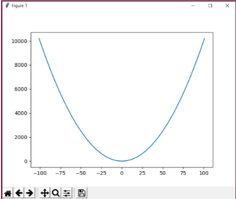
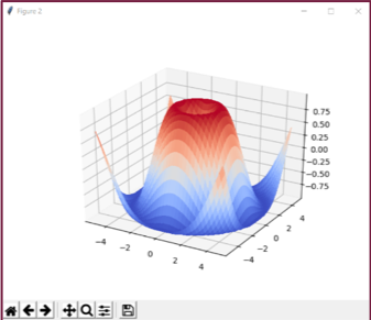
Matplotlilb provides 2-d charts, but other packages built upon Matplotlib provide 3-d charts, as per the following example.
>>> from mpl_toolkits.mplot3d import Axes3D
>>> import matplotlib.pyplot as plt
>>> from matplotlib import cm
>>> from matplotlib.ticker import LinearLocator, FormatStrFormatter
>>> import numpy as np
>>> fig = plt.figure()
>>> ax = fig.gca(projection='3d')
>>> X = np.arange(-5, 5, 0.25)
>>> Y = np.arange(-5, 5, 0.25)
>>> X, Y = np.meshgrid(X, Y)
>>> R = np.sqrt(X**2 + Y**2)
>>> Z = np.sin(R)

>>> surf = ax.plot_surface(X, Y, Z, cmap=cm.coolwarm, linewidth=0, antialiased=False)
-
There are many examples on the web that illustrate Python’s graphing capabilities. Rest assured that you can create all the charts you’ve grown accustomed to with MATLAB.
-
Additional packages provide the ability to make interactive charts, to add filters, and to create dashboards. Plotly, mentioned earlier, is an open-source package that interfaces with both MATLAB and Python. In particular, have a look at plotly.js, which is the plotting component of Plotly. Plotly.js is built on top of D3.js and thus provides a rich set of dynamic, interactive charts. With Plotly.js, you get all the features of D3.js, but you get to work in the MATLAB and Python languages.
-
For statistical charts, you’ll want to check out the seaborn package, which is built on top of Matplotlilb. The seaborn gallery has a collection of charts that are readily available to you.
-
Lastly, as an open source language Python enjoys a wide audience of contributors. Chart types for many specific data sets have been contributed to the library of packages. Have a look at Yan Holtz’s Python Graph Gallery for an overview of the chart types available in Python.
Object-Oriented Programming in Python
At this point of the article we’ll dive a bit deeper into the Python programming language. We’ll discuss namespaces, scopes, and then classes. Each of these differs from the MATLAB model, and you need to be aware of the differences.
Namespaces and Scopes
Let’s start with namespaces and scopes, as these concepts are important prerequisites for understanding classes.
-
A namespace is a mapping of names to objects, typically implemented as a dictionary. Examples include built-in names, exception names, global names of a module, and local names of a function.
-
Namespaces are implemented (currently, anyway) as dictionaries. The dictionary keys are variable names, and the associated values are the objects that the names point to.
-
In Python, a global namespace refers to the top-level space of a single module. The global namespaces of two or more modules are not shared.
-
Attributes of an object are effectively a namespace.
-
A scope is a textual region of a program where a namespace is directly accessible.
-
At any time during program execution, at least three scopes are in effect. From the innermost scope to the outermost, these are:
-
The innermost scope is that of any embedded function (a function embedded in an enclosing function). When Python is trying to resolve a reference, this innermost scope of local names is searched first.
-
The scopes of enclosing functions, containing non-local, but also non-global names is the second-most inner scope. When resolving references, this scope is searched second.
-
The next to last scope (the middle, or global scope) contains a module’s global names.
-
The outermost scope (searched last) is the namespace containing built-in names.
-
-
Variables can be declared global, in which case they will reside in the middle scope. These variables will not be shared across modules.
-
Within the four scopes, variables flow from the outer scopes into the inner scopes. That is, a variable declared in an outer scope can be referenced in an inner scope. The converse is not true; variables defined in an inner scope cannot be referenced in an outer scope. To alter this latter behaviour, variables in an inner scope can be declared nonlocal, whereby they will pass by reference into any outer scope.
Classes
For programming projects of non-trivial size, the use of classes is considered standard practice. MATLAB provides a sophisticated class model that, while offering programmers tremendous capabilities, is difficult to learn. Python’s class model is much simpler, offers fewer capabilities, but is easier to learn. Let’s have a look.
In the following, we’ll make no attempt to explain object-oriented programming; we are instead assuming you have covered this topic elsewhere. We’ll provide an outline of what Python offers, from as usual, the perspective of a MATLAB programmer.
In Python everything is an object; in MATLAB most but not all things are objects.
Let’s look at a few simple Python examples of variables. Consider the following:
>>> x = []
>>> x?
Type: list
String form: []
Length: 0
Docstring: Built-in mutable sequence.
As the above shows, even the [] construct creates an object. In this case, variable x is a list object. Or consider how a variable containing an integer has a class attribute:
>>> x = 5
>>> x.__class__
<class 'int'>
Classes are defined with a straightforward syntax. In the following example code, we define a class, a docstring, an instantiation method, and then two class methods:
class MyClass:
        """A sample class definition"""         # Like MATLAB's H1 line

        def __init__(self):      # A constructor
            self.mydata = []

        def method1(self):
            self.mydata = 3.14159

        def method2(self):
            self.mydata = 3.14159 / 2
Class objects support only two kinds of operations: attribute references and instantiation. Let’s look first at attribute references. Consider the following class definition which defines one attribute and one method:
class MyClass:
        """Doc String"""
        x = 3.140

        def f(self,StringToPrint):
        print(StringToPrint)
You’ll need to save the above into a .py file. You can choose any name for the file; let’s use simple.py. Back in the Python console window, we can type the following:
>>> import simple
>>> obj = simple.MyClass()
>>> obj.x
3.14
>>> obj.f('test')
'test'
Both the attribute and the method are referenced with the same notation. Use of the variable ‘self’ as the first argument to the above method is only a convention; this is, however, the standard convention.
Now let’s look at an instantiation operation. Python uses a specifically named
method for instantiation, called __init__, as per the following example:
def __init__(self, day, activity):
    self.weekday = day
    self.activity = activity
When an __init__ method is placed into a class definition, it is automatically
invoked when the class is first instantiated.
Python supports class inheritance. The syntax is simply:
class SubClassName(BaseClassName):
In the above, BaseClassName must be in scope. If it is not, one can instead use:
class SubClassName(ModuleName.BaseClassName):
Subclass methods may either override or extend base class methods of the same name. To call a super-class method from a subclass, use super(). For example, if a parent class has a method called invite(), the subclass can reference the method with super().invite().
Python supports both class (static) and instance variables. The location where variables are defined in a class, rather than the use of keywords, dictates whether a variable is a class variable or instance variable. E.g.,
def MyClass:
    ClassVar = 3.14     # Class, or static variable

def __init__(self):
    self.InstanceVar = 3.14159     # Instance variable
Static variables should be used with care. If you create two instances of the above class and use one of them to alter the value of ClassVar, that value will then appear also in the second instance.
Python also supports static methods. This introduces the topic of Python’s class decorators, which we consider to be an advanced topic best saved for later. But for now, know that Python supports both static and instance methods.
In MATLAB, a class resides in a file of the same name. In Python, multiple classes can be defined in one file, and that file can take any name. More generally, a class can be defined anywhere, e.g., inside of a function or an if statement (not that you would do that, of course). Classes can be embedded within one another, with the inner class having access to the outer class namespace. The author of Python, Guido van Rossum, maintains a blog where he has an interesting discussion of this topic.
There are some significant differences between the MATLAB object model and Python’s. Here are the biggest ones:
-
MATLAB provides private attributes (for both properties and methods); Python does not.
-
Further, MATLAB provides numerous property attributes such as Abstract=true. Python offers none of these.
-
MATLAB also offers object events, or listeners; Python does not.
-
MATLAB requires that a file can hold only one class; Python has no such restriction.
There are many more differences between the MATLAB and Python object models. In general, the Python model chooses simplicity over sophistication; vice-versa for MATLAB. Which model is the best choice will depend upon your programming needs.
Mutability
Python considers everything to be an object. Once initiated, some objects allow their state to be changed, meaning they are mutable. Other objects prohibit state changes; these objects are immutable. Knowing which classes are mutable and which are not is important. Here’s a reference list:
-
Mutable classes: list, set, dict and byte array
-
Immutable classes: bool, complex, float, int, str, tuple and frozenset
It may seem strange that Python defines so many immutable classes. But beyond the primitive data types (bool, complex, float and int) only three classes are immutable. And of those three, the tuple class allows its contents to contain mutable objects.
Copy That
To close out this chapter, let’s discuss an interesting, and likely unexpected, feature of Python: the language provides three mechanisms for copying variables. We think it’s best to inform you of this now, so that you don’t learn about this after tripping over it.
Suppose you have a list referenced by the variable x. If you then create a new variable y with the operation y=x, the new variable y simply points to the original list; the variable y does not reference a new copy of the list. This is an important concept to master as it effects all Python data types. On assignment, Python will bind two objects together rather than make a copy. Consider the following:
>>> x = [0, 1, 2, 3]
>>> y = x
>>> x[0] = 99
>>> y
[99, 1, 2, 3]
By updating x we also updated y, because y was bound to x. From the MATLAB perspective, x and y are similar to handle objects; unlike MATLAB, Python defaults to this behavior.
When necessary Python will allow you to make a true copy. But there are two flavors of true copies. The first is called a shallow copy. For simple objects like a list that don’t contain nested objects, the shallow copy is all you need.
>>> import copy
>>> x = [0, 1, 2, 3]
>>> y = x.copy()
>>> x[0] = 99
>>> y
[0, 1, 2, 3]
When you are trying to copy more complex objects, such as a user-defined object whose attributes reference other objects, you will need a deep copy of the list. In this third case, use x.deepcopy() instead of x.copy().
An important exception to binding is in making array slices. When an array is sliced, the returned object is a new object, not a view into the original object. E.g.,
>>> a = list(range(5))
>>> b = a[2]     # A slice, which is not bound to variable 'a'.
>>> b
2
>>> b = 99     # Change the value of b.
>>> a
[0, 1, 2, 3, 4]     # Variable a is unaffected.
Biggest Differences
Now that you’ve seen Python’s primary data types and control structures, let’s catalog the major differences between the Python and MATLAB languages. Here are the items that made our list. If you are going to program in the Python language, you’ll want to spend some time studying these topics further.
-
Python array indexing: zero-based rather than one-based, and square brackets rather than parentheses.
-
List comprehensions: there’s really no equivalent in MATLAB.
-
Iterables, iterators and generators: important features of the Python language. MATLAB does not offer these features, although you can code them yourself.
-
Mutability: this is an important concept in Python. This same concept exists in MATLAB, but programmers are largely shielded from and thus often unaware of it.
-
Bindings, shallow copies and deep copies: by default Python treats objects like MATLAB handle objects.
We have now covered the primary Python data types and control structures. In the
third and last chapter of this article, we’ll look at the expansive Python
ecosystem.
The Python Ecosystem
As a MATLAB programmer you may be a little nervous about Python at this point. We covered the primary data types and built-in functionality, but said nothing of matrices, multi-dimensional arrays, array operations or vectorization. We haven’t even mentioned common mathematical operations such as matrix inversion, eigenvalue computation, interpolation or the like.
The closest we came to any of those discussions was to introduce lists, and we noted that lists are like MATLAB’s cell array. But we also noted that Python lists do not support matrices or higher-dimensional arrays. The core Python language simply does not replicate the MATLAB features you rely upon. But fear not, for Python is designed to be an extensible language and its ecosystem provides the data types and functionality you’ve been wondering about.
The Python ecosystem, the libraries, IDEs and tools that complement the Python language is vast. We noted earlier that learning the Python language requires a substantial, yet limited, amount of your time. In contrast, discovering all that is available in the Python ecosystem is, well, good luck with that. In the following sections, we will introduce you to those portions of the ecosystem that are likely to be of value to you. We cannot cover everything that might be of interest to you, but we’ll start the conversation and provide you with links to additional material.
Integration with Source Code Control
Python itself does not integrate with source control systems, but many of its IDEs do. PyCharm, for example, has an intuitive interface to more than ten source control systems, including GitHub, CVS and Subversion. In PyCharm, go to File->Settings->Version Control and choose your SCC of preference. Once your settings are made, there’s a VCS menu on the PyCharm toolbar. It’s that easy. Note that file names within the project listing (left side of the PyCharm window) are color coded to reflect their SCC state.
Back to Modules and Packages
As mentioned earlier, a searchable list of 150,000 Python packages is available at the Python Package Index. Before reinventing the wheel, search through the index to see if someone has already published the code you need. Downloading packages is easy, and your IDE may make it trivial for you. Let’s talk now about importing modules and packages into your Python workspace.
-
In Python, a module is a .py file; an organizational unit.
-
A package is a collection of modules in a directory. A package will also contain a file called init.py.
-
The module name is the name of the file (minus the .py extension).
-
A module typically contains a set of function definitions but may also contain executable statements; these statements initialize the module and are executed only the first time the module is imported.
-
The base workspace is referred to as the main module.
-
An import introduces the referenced module name to the current symbol table and executes any executable statements at the top of the module.
-
Each module has its own symbol table. That table is called a global table and is used by each function in the module. The scope of a global table is its module; modules cannot see one another’s global table.
-
Packages provide a further separation of scope. Whereas modules each contain their own global variable scope (thus shielding each other from variable and function name collisions), packages shield one another from colliding module names.
- Modules are imported with the import command.
>>> import statistics as statThe above will import (register) the statistics module, abbreviated as stat. This does not actually load the statistics functions into the current workspace. Rather, the command registers the names of the functions in the module, and makes them available with, e.g.,
>>> avg = stat.mean(x) - When you import a module, all of the functions it contains will be
registered. This means that a .py file can contain multiple functions, and
all will register. Specific functions in a module can be imported with,
e.g.,
>>> from statistics import meanThe above will register the mean() function but will not register the module name.
- On startup, Python loads the modules of its standard library. The following
list comprehension will print the set of currently imported modules:
>>> import sys >>> [str(m) for m in sys.modules] - To determine which functions are defined in module, use the built-in dir()
function. For example:
>>> import sys
>>> dir(sys)
We’ll skip the output here, as it is lengthy.
To install packages, a utility called ‘pip’ is recommended. Here’s how to use pip to install the matplotlib package.
Find pip.exe on your computer; this executable should have installed as part of the Python install. Add that directory to Windows’ path variable. Just type ‘Edit Environment’ in the Windows task bar and you’ll find the variable editor. See the following link for instructions.
In a command prompt window (Windows, not Python), enter the following:
pip install matplotlib
pip freeze
Occasionally you’ll want to upgrade the installed version of pip. To do so, enter (in a command prompt window):
pip install --upgrade pip
With thousands of available packages, one might expect that updates to various packages happen all the time. However, only one version of a given package can be installed in the same Python instance; that is, a specific package name can be imported only once, even if there are multiple versions available. To enable testing of new packages, and to enable version-dependent programs to run with outdated packages, Python allows for virtual environments. A virtual environment is just a directory tree containing a Python installation, along with a set of version-specific packages.
Python itself can create virtual environments (also known as venvs), using the command venv. Likewise, many IDEs can create such environments. If you are using a venv, be aware that pip installs packages and modules local only to that venv. That is, if you download a package specific to a venv, that package will not be included with, or available to, the next venv that you create.
Virtual environments are very useful and provide a feature missing in MATLAB: an ability to switch between different module and package versions for testing or debugging.
Path Management
You may have noticed that we’ve not mentioned path management. No doubt you are aware that path management is important to MATLAB: classes, functions and scripts must reside on the path, and file naming conventions must be followed.
In contrast, Python path management tends to be simpler. The path will likely be shorter, more easily managed, and once a module is imported, all of its functions are directly accessible. By default, the packages that you install with the pip utility will reside in a single folder under the Python installation folder. To list your specific site folder(s), perform the following command:
>>> import site; site.getsitepackages()
If you know the name of a specific package you’ve already installed, you can obtain information about that package, including its installation directory. Use the following command entered into a Windows command window to obtain information about a package named, e.g., package-name:
pip show package-name
If you are using a virtual environment, the venv tool or your IDE will create
its necessary virtual environment folders and update the path variable
automatically.
Here are the basics for viewing and modifying the Python search path.
-
The Python search path is saved in a variable called sys.path.
- To view the directories currently on the path, you can use the
following:
>>> import sys; print(sys.path) - To append the system path, use, e.g.,
>>> sys.path.append('C:Temp')
NumPy
We promised several times to show you how Python supports matrices, higher-dimensional arrays, and associated numeric and scientific computations. That time has arrived.
One of the design objectives for the core Python library was, and remains, simplicity. Matrices and higher-dimensional arrays are thus provided by add-on packages. By far the most popular package to provide an array feature is NumPy. The NumPy package bills itself as the fundamental package for scientific computing with Python.
We’ll cover some NumPy basics, just to show you that MATLAB’s array features are available in Python. But for a full discussion of NumPy, you’ll want to visit the official NumPy website.
To begin, install NumPy.
C:> pip install numpy # Enter from a Windows terminal
We’ll focus on the a NumPy-specific data type called ndarray, which has an alias called array. This data type provides storage for a multi-dimensional array of homogeneous elements. Let’s first create and print a 1-d array of integers:
>>> import numpy as np
>>> a = np.array([1,2,3]) # Note that we input a list.
      # Omitting the brackets generates an error.
>>> print(a)
[1 2 3]
Create and print a 2-d array of integers. There are numerous ways to create arrays in NumPy, and we’ll explore a few of those.
>>> a = np.array([ (0, 1, 2, 3),
...                (4, 5, 6, 7) ])
>>> print(a)
[[0 1 2 3]
[4 5 6 7]]

>>> a = np.arange(8).reshape(2,4) # Equivalent to the above

>>> a[0,0] # Single brackets now; different from core Python
1

>>> a[0,1] = 99
>>> print(a)
[[1 99 3]
[4 5 6]]
The array() function transforms sequences of sequences into two-dimensional arrays, sequences of sequences of sequences into three-dimensional arrays, and so on.
NumPy provides several functions that will immediately be familiar, for example: zeros(), ones(), and linspace().
Regarding operations on arrays, NumPy performs elementwise computations by default; linear algebra operations are obtained through special functions.
>>> a = np.array([ (1,2,3), (4,5,6) ])
>>> a += 1 # An in-place operation, equivalent to a = a+1
>>> print(a)
[[2 3 4]
[5 6 7]]

>>> a *= a # Element-wise multiplication, equivalent to a =
a*a
>>> print(a)
[[4 9 16]
[25 36 49]]
Recall from earlier that Python uses the ‘+’ symbol to concatenate arrays, even numeric ones. NumPy overrides that behavior, giving you elementwise operations. E.g.,
>>> a + a
array([[ 8, 18, 32],
       [50, 72, 98]])
Now let’s look at a matrix product, using the @ operator. Rather than save and
then print() the result, we’ll skip the save and allow Python to print to the
screen.
>>> a = np.array( [[1,2]
                   [3,4]])
>>> b = np.array( [[2,3]
                   [4,5]])
>>> a @ b
array([10, 13],
      [22, 29])
NumPy has dozens of functions with which to perform the usual array operations you would expect of an analytics library. You can query an array size, reshape an array, extract elements or slices, compute statistics such as cov, mean, std and var. With NumPy you can perform linear algebra operations such as transpose, inverse and multiplication. You can compute eigenvalues. You can sort and filter arrays. Logical operations include the familiar any(), all() and where() operations.
By default, NumPy will operate on arrays element-wise. This is a departure from MATLAB’s vectorized operations. However, NumPy provides a vectorization feature via its vectorize class. As a simple example, suppose you have a function called add.py which inputs two numbers, adds them and returns the result. Below is the function, and how you would vectorize it.
>>> import numpy as np
>>> def add(a, b):
... return a+b

>>> add_v = np.vectorize(add) # Returns a function
>>> add_v([1, 2, 3], [4, 5, 6]) # Add two vectors
array([5, 7, 9])
While it’s not a core topic of this article, we should mention that NumPy offers a tremendous performance benefit to numeric calculations. Calculations that you might compute in pure Python can run 10x to 100x faster using NumPy. This performance improvement results from several key features of NumPy. Consider the simple act of adding two lists. In pure Python, each element of the list will be a pointer to an object, a float or an int, for example, with all of the attendent overhead of processing those objects. In NumPy, those lists will be reduced to arrays of a homogenous data type, with far less processing overhead. Secondly, many NumPy functions are implemented in the C language, compiled for speed. And thirdly, with NumPy, high-level Python for-loops get pushed down into the C libraries, with the latter being far faster than the former.
NumPy has much more to offer; we simply cannot cover all of its capabilities
here. But a bit of good news for you: with a MATLAB background you’ll find that
the NumPy documentation is familiar, and once you read
through its documentation you’ll feel much more at ease with Python. And if you
don’t particularly like the NumPy language syntax, keep reading to the Pandas
section. Pandas is built on top of NumPy and provides a syntax you will be much
more comfortable with.
SciPy
The NumPy package is built upon the core Python language and provides an N-dimensional array type. The SciPy package is built upon the NumPy package and provides a tremendous breadth of mathematical, scientific and engineering algorithms. SciPy is actually one component of a larger ecosystem of packages, including: NumPy, Matplotlib, IPython, Pandas and numerous others. Generally, when you import SciPy, you’ll want to import NumPy. Depending on your needs, you’ll import the other packages as required. When you import SciPy and its friends, you are creating a Python computational environment that is similar to what you are accustomed to with MATLAB.
SciPy provides a collection of modules targeted toward science and engineering. SciPy modules include algorithms for linear algebra, FFTs, integration, interpolation, optimization, signal and image processing, differential equations, statistics and more. SciPy also extends Python’s computational features by providing advanced charting, database interactivity and parallel processing. SciPy can even read and write MAT-files.
Be aware that some SciPy functions also appear in NumPy, and there will be non-trivial differences between them. This duplication exists for NumPy backward compatibility reasons. A good guideline is to use NumPy for its multi-dimensional array type, and SciPy for its algorithms.
The ecosystem built on SciPy is vast. Fortunately, the SciPy team maintains an extensive list that is categorized by scientific discipline and computational topic. We encourage you to browse through the offerings. But first, let’s take a quick look at SciPY.
To begin, install SciPy.
C:> pip install scipy # Enter from a Windows terminal
Let’s solve linear system [A]{x} = {b}, where [A] and {b} are given as:
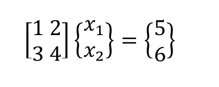
>>> import numpy as np
>>> from scipy import linalg

>>> A = np.array([[1, 2], [3, 4]])
>>> b = np.array([[5], [6]])
>>> x = np.linalg.solve(A, b)
>>> print(x)
[[-4, ],
[ 4.5]]
Check that the solution is correct. Compare the multiplication of
[A]{x} to {b}.
>>> Ax = np.dot(A,x)
>>> tf = all(np.equal(Ax, b))
>>> print('Solution matches:', tf)
Solution matches: True
The SciPy package has extensive functionality, and extensive documentation. The online documentation at scipy.org is excellent, and you’ll eventually find yourself spending time there.
Pandas
Building on NumPy and SciPy is the Pandas package. Pandas is all about data analysis and modeling. The pandas website states, pandas has ‘the broader goal of becoming the most powerful and flexible open source data analysis / manipulation tool available in any language.’ Note that the name pandas, by convention, is written in all lowercase.
If you rely upon MATLAB’s @dataset or @table classes, or if you have coded your own version of these classes, or if you need to analyze and model data, you’ll want to explore the pandas package. Pandas offers both a Series class for 1-d data, and a DataFrame class for 2-d data. Each of these classes comes with labels, indices, and broad functionality for data import and export, data cleansing, analysis and modeling, charting and numerous other tasks.
Pandas depends upon and extends the NumPy package. Pandas does not depend upon, but interoperates with, SciPy. It’s quite possible that a lot of code you had to write before in MATLAB simply goes away now, as the code has been written for you in Python’s NumPy/SciPy/pandas ecosystem.
Development of pandas began in 2008 at AQR Capital Management, and the library was open-sourced in 2009. Pandas does many of the things that you’ve grown accustomed to in MATLAB. It is difficult to reduce the list of pandas’ capabilities to a set that might be most important to you, but here’s an attempt.
Pandas can read data from a wide variety of data sources, including CSV and other delimited files, Excel, databases, HDF5, HTML and JSON. Pandas has facilities for storing variable-frequency timeseries data, both 1-d and 2-d, and for managing timeseries data with operations such as filling, converting frequencies, and date shifting. As with NumPy, pandas provides indexing and slicing of your data, and numerous relational operations such as group by, join and merge. Data and axes can be labeled and indexed. Pandas provides facilities for data analysis and modeling, and pandas interoperates with the functions provided by SciPy.
Let’s try an example using pandas. Suppose you notice a news article about the Consumer Price Index (CPI) for U.S. Housing and want to explore some of that data. An online search leads you to the Bureau of Labor Statistics and to a set of csv files on their website. In the following code, we’ll read the CPI data, explore it, reduce its frequency from monthly to annual, and then chart it.
To begin, install pandas.
C:> pip install pandas # Enter from a Windows terminal
Next, let’s read the online data, and take a quick look at the contents:
>>> import pandas as pd

>>> URL =
'https://download.bls.gov/pub/time.series/cu/cu.data.12.USHousing'
>>> df = pd.read_csv(URL, sep='t') # df is short for
DataFrame
>>> df.head()

series_id year period value

0 CUSR0000SAH 1967 M01 30.5
1 CUSR0000SAH 1967 M02 30.5
2 CUSR0000SAH 1967 M03 30.5
3 CUSR0000SAH 1967 M04 30.6
4 CUSR0000SAH 1967 M05 30.7
Pandas was able to read the csv file and place it directly into a DataFrame. Note that Pandas added the first column (a row index) automatically. We won’t need the series_id column, so let’s drop it. Also, it turns out that the CPI data is rather sparse before 1940, so let’s keep only years 1940 and later:
>>> df = df.drop('series_id', axis='columns')
>>> df = df[df.year >= 1940]
The column labeled ‘period’ denotes a month. E.g., M01 is January, M02 is February, etc. Let’s use some of panda’s built-in SQL functionality to group the CPI indices by year, taking the mean CPI across the months of each year. Note how we are chaining operations together:
>>> df = df.groupby(['year']).mean()
Finally, let’s clean up the column labels and plot the data:
>>> df = df.rename({'value':'Mean CPI'}, axis='columns')
>>> df.plot()
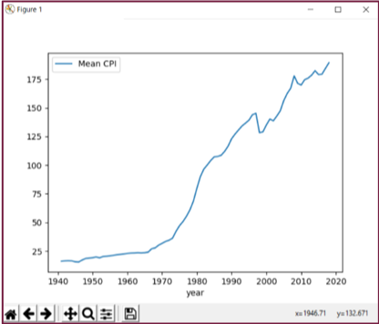
Plotting the data provides the figure above. Several comments are warranted here. First, the pandas library was able to successfully load a remotely-hosted data set that we did not even bother to pre-inspect. Pandas placed the data into its DataFrame object, automatically included labels and inserted a row index. Using pandas’ functionality, we were then able to remove unwanted data, both rows and columns, reduce it to an annual frequency, clean up the labels and plot. We used a total of nine commands.
While pandas’ syntax differs from MATLAB’s, the commands we used to analyze the CPI data should feel familiar. Pandas has a tremendous amount of functionality that we’ve not touched upon, but hopefully we’ve demonstrated that the combination of Python/NumPy/SciPy/pandas provides an analysis environment similar to what you use with MATLAB.
Full-Stack Python
Full-Stack Python refers to the design and deployment of web-based applications with significant server-side functionality. Using nothing but Python and supporting Python-based libraries, one can create complex web apps which integrate into traditional websites and back-ends. Python libraries are available for web frameworks (e.g., Django and Flask) and front-end user interfaces (e.g., Plotly Dash).
As an example, one of the authors of this article (Patterson) has written a web application for stress-testing trading portfolios comprised of options, futures, and swaps. This app employs complex mathematical modeling, large data sets, extensive computations, and a sophisticated user interface. The app is written completely in Python. A screen shot of the app is shown below. For a demo of the application or to inquire about licensing, please contact its author.
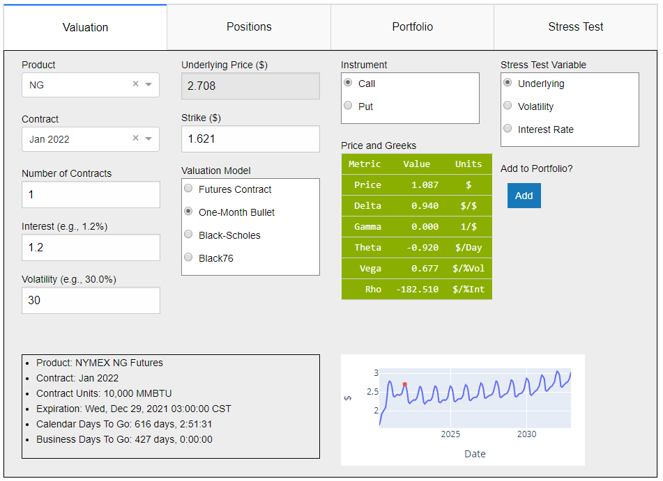
As discussed above, Python can handle both the front-end and back-end of a web app, and also everything in between, such as analytics and database access. Rather than belabor this topic, we’ll refer you to an excellent online resource called, appropriately, Full Stack Python written by Matt Makai.
MATLAB and Python, Together
The next item in the Python ecosystem that we’d like to introduce is one that will be familiar to you: MATLAB. It may seem odd to include MATLAB as part of the Python ecosystem, but the two languages play supporting roles to one another. If you happen to own a MATLAB license, why not employ it as part of your Python programming efforts?
Python can call MATLAB scripts and functions. In fact, The MathWorks has published an API for Python package that you can import into your Python workspace to facilitate such calls. The package enables you to launch MATLAB from a Python script, transfer data to the MATLAB instance, invoke functions, and return results.
Why, you might ask, would you want to call MATLAB scripts from Python? We think there are several use cases. The first is one of deployment. Suppose you have analytics functionality built in MATLAB but want to deploy those analyses on the web. Python has, though we’ve not discussed it here, state-of-the-art GUI toolkits that can easily be deployed on AWS, the Google Computing Platform or otherwise. You can construct your analytics front-end in Python, allowing it to communicate with your MATLAB-based back-end library.
A second use case is one of developer efficiency. The knowledge you’ve obtained in MATLAB continues to be valuable: you may have an extensive library of M-code that you cannot justify recreating, or perhaps you have a wealth of experience with a MATLAB toolbox and don’t want to relearn that in a new language. In these situations, you’ll want to retain your work in MATLAB even as you branch out in Python.
Just as MATLAB is part of the Python ecosystem, the reverse is also true: Python is part of the MATLAB ecosystem. This latter perspective may be the one that best applies to you. We’re happy to report that you can experiment with Python as a programming language without leaving your established MATLAB-based platform.
Your MATLAB scripts can call newly developed Python code, and the MathWorks has published functions to facilitate that interaction. Why, you might ask again, would you want to call Python scripts from MATLAB? The answer is that Python does some things very well, such as reading online data sources and databases. The possibilities here are unlimited and depend upon your specific needs. As we stated in the beginning of this article, knowing both languages will provide you with opportunities not previously imagined.
Integrated Development Environments (IDEs)
Let’s return to a topic that we first discussed at the very beginning of the article: IDEs. There are at least twenty IDEs to choose from. One called IDLE ships with the Python download but is limited in functionality. If you choose to begin developing with Python, you’ll want to upgrade to one of the other choices.
The authors sometimes use the community (free) version of PyCharm. We also use the Professional (not free) version. PyCharm provides code completion, code formatting, syntax highlighting, runtime error checking, project navigation, debugging, and a slick interface. PyCharm integrates with several source control libraries, unit testing frameworks, databases, virtul environments and the PyPy package management library. PyCharm also integrates with the scientific libraries we’ve discussed in this article and supports the IPython magic commands. PyCharm is every bit as sophisticated as the MATLAB IDE, and even more so.
If you happen to use Visual Studio, you can stay with that editor as it supports Python. And if you’re more of a command-line person, have a look at IPython, which is a Python prompt with auto-completion, history and shell capabilities.
Lastly, we mentioned earlier that an IDE called Spyder is available, and it provides a programming environment similar to MATLAB’s. From the Spyder website:
Spyder is a powerful scientific environment written in Python, for Python, and designed by and for scientists, engineers and data analysts. It offers a unique combination of the advanced editing, analysis, debugging, and profiling functionality of a comprehensive development tool with the data exploration, interactive execution, deep inspection, and beautiful visualization capabilities of a scientific package.
Spyder has many features you’ll recognize. Advanced editing features include syntax highlighting, real-time code analysis, code cells, on-demand completion, tool tips, window-splitting and more. The IDE includes a debugger and profiler, interactive execution, a variable explorer, data explorer and visualizer, and version control. The Spyder IPython console window will assist you with function tips, automatic indentation, syntax highlighting and command history. You can open multiple console windows, and each will operate independently of the others.
Spyder is similar to PyCharm but targeted to data scientists and analysts. Spyder even knows about and integrates with NumPy, SciPy, and Pandas.
Pictured below is Spyder along with our earlier example of using Pandas to visualize BLM data. The window on the left is the editor displaying our code. To the bottom-right is the Python console, along with integrated graphics. At the top-right is the variable explorer; superimposed upon it is the output DataFrame which we obtained by double-clicking on that variable in the explorer window.
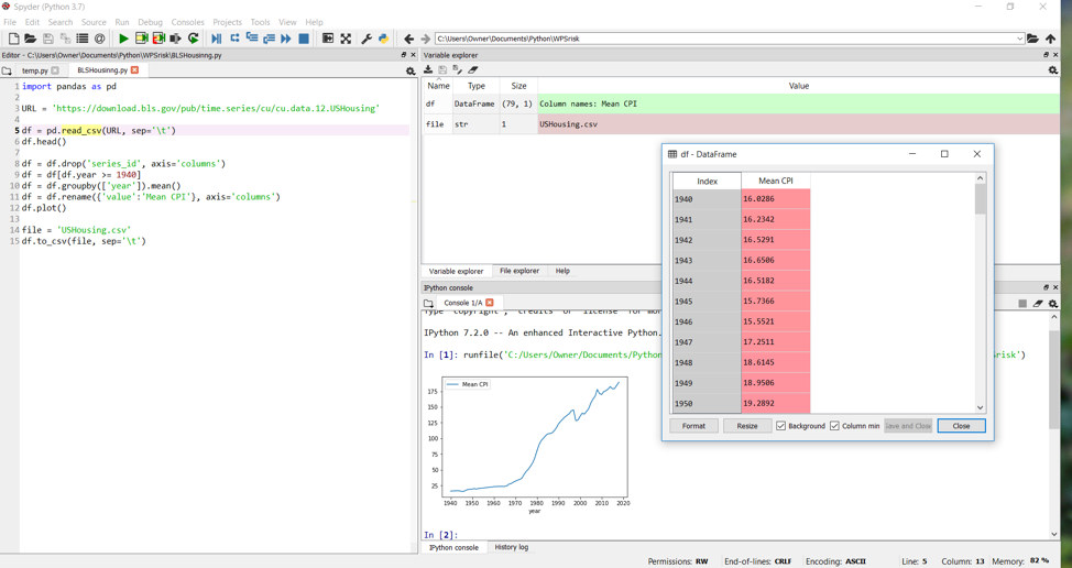
Spyder is written in the Python language, is open source and is free of charge.
Anaconda
Spyder is a core component of a Python distribution called Anaconda. The Anaconda distribution mimics a MATLAB installation, in that it provides a complete computing environment: the Python engine, all of the packages we covered earlier, a package manager, the Spyder IDE, and more. With the Anaconda distribution, you no longer have to go shopping for all of these various components. Anaconda gives you the best of breed in each category, all targeted toward data science.
In addition to Python, Anaconda includes Jupyter Notebook, which is a Python engine that allows you to create interactive notebooks of Python code, output of that code, any associated charts, and inline descriptive text. These notebooks are great for teaching and collaboration.
Anaconda is free and open source. In addition, the Anaconda Cloud provides you with online storage to collaborate on modules, packages, notebooks and environments. The Cloud is free for publicly-shared projects. For a monthly fee you can host private collaborations.
With more than six million users, Anaconda is a popular distribution worthy of
your attention.
Closing
If you have read this far, you must be interested in Python. There’s more to learn, of course, but if you have absorbed the concepts you’ve just read about, you are already functional with the Python language.
If you did not perform the installations and code snippet executions provided throughout this article, a good next step would be to read through the article again, performing all of the installations and examples. When we first mentioned IDEs (back on page 3) we mentioned that you should perhaps wait to choose an IDE. But now’s the time. If you want to put together your own Python computing environment, you can download Python, the packages you need, and the IDE of your choice. Alternatively, you can skip all of that and just download Anaconda.
Two documents are particularly important for your continued study. The Python Library Reference will tell you about the functions in the Python Standard Library. We’ve touched on many functions in this article, but the Library Reference is the definitive guide. Secondly, the Python Language Reference is a comprehensive document that will tell you everything about the language’s design, syntax and semantics.
You absolutely should visit the Python Software Foundation home page. From there you can find the above two documents, tutorials, how-to guides, code examples, installation guides and much more.
If you are more of a book reader, there are numerous books worthy of your time and dollars. On the topic of Python and data science, one book that we recommend is O’Reilly’s Python for Data Analysis, written by Wes McKinney, creator of the pandas library. This is an incredibly well-written and thorough book, an enjoyable read. You can purchase a digital version and then cut-and-paste examples from the book into your Python interpreter. Or better, you can follow along in the book with an accompanying Jupyter Notebook that provides interactive examples for you.
We thank you for your time, and we hope you have found this article worthy of
that time. If you have feedback, if you have found typos, incorrect statements,
important omissions, or if you have suggestions for improving this document,
we’d like to hear from you. Our biographies and contact information are listed
below.
Author Biographies
Michael Patterson has worked in commodity trading for twenty years, with roles in technology, fundamental analysis, business intelligence and risk management. Michael lives in Tulsa, OK with his wife and two children. Michael can be reached via his LinkedIn profile or by email at michael.patterson@demextech.com.
Andrew Janke is a software developer with over a decade of experience building MATLAB-based systems for financial analysis applications. Andrew specializes in building data analytics platforms that integrate multiple languages and technologies, including MATLAB, Java, and SQL. He can be reached at his website, LinkedIn profile or by email at andrew.janke@demextech.com or andrew@apjanke.net.
Michael and Andrew currently work at Demex Technologies, where Michael is Director, Commodity Analytics and Andrew is Director, Quantitative Systems. Among its products, Demex Technologies provides to its clients an online platform for researching and quoting complex commodity and weather-based financial derivatives. Not surprisingly, the platform is written in a mix of languages, including MATLAB and Python.
The Demex Group
The authors of this article are founding members of The Demex Group, a firm which helps clients adapt to the impacts of changing weather and climate. A quick background on The Demex Group will help you understand why we’ve taken the time to write this article for you.
We help our clients quantify their business exposure to weather and climate risks, and we facilitate the transfer of those risks to third parties. We do this by providing our clients access to algorithms that help them discover and mitigate their risk exposures. Our algorithms are hosted on a sophisticated, web-based platform comprising nearly one hundred man-years of efforts. To no surprise, this platform is written largely in the MATLAB and Python languages.
Analytics and technology are the core of our business, and client relationships
are the foundation of that business. We share our platform and our analyses
with our clients, and in so doing we empower them and help protect them from
weather and climate risks. This article is just one small component of that
effort: we’d like to share with you the knowledge we’ve acquired in our work.
Contributors
Numerous people have graciously offered reviews, corrections and contributions to this document. We wish to recognize and thank them for their time and talents. Their names, with links to their LinkedIn profiles are:
We would like for this list to grow. Please consider adding to the article. A list of suggested new topics resides on the article’s GitHub public repository.